unstructured search, but smarter

i finally made a quantum post

introduction

It seems there’s been a paradigm shift in the way popular media talks about quantum computing. Initially pessimistic, even revolutionary tech figures like Jensen Huang have turned heel on what they now believe to be the viability of large-scale quantum computers in the near future. Yet today there are several compelling reasons to take quantum seriously; the “elevator pitch” is not exclusively an appeal to authority. I won’t dive into those reasons here, but if you’re curious why I think this is such an exciting area of computer science, feel free to email me and I’d be happy to explain in detail.

For those already interested in quantum, demonstrating quantum advantage remains paramount. After all, quantum computing was originally sold as a model that could deliver dramatically faster speed‑ups across a wide class of problems. In some cases, these speed‑ups are exponential: for example, John Watrous’s excellent video on quantum‑query algorithms in IBM’s “Fundamentals of Quantum Algorithms” series. However, many of these algorithms feel somewhat artificially constructed to highlight extreme cases. Today, we’ll discuss an algorithm whose speed‑up is more modest in scale but applies to a much broader class of problems.

the problem itself

Given black-box access to a function $f : \{0, 1\}^n \to \{0, 1\}$, output a marked input $\mathbf {x}^*$ such that $f(\mathbf{x}^*) = 1$, if one exists.

here, black-box access means that we can only interact with the function $f$ via querying $f$ on bit-strings in $\{0, 1\}^n$. we do not have access to any algorithm or circuit that can compute said function. Assume that $N := 2^n$.

a classical lower bound

the best known classical algorithm for this setting of problem is unfortunately no better than brute-force. given that there are $N$ $n$-bit binary strings, this provides a run-time of $\Omega(N)$.

querying a function quantumly

operations in the quantum world are mostly¹ governed by unitary transformations and measurements. querying a function $f$ quantumly is specified as follows

$$ \begin{align*} \ket{x} \ket{y} &\substack{\mathbf{U}_f \\ \mapsto} \ket{x} \ket{y \oplus f(x)} \end{align*} $$

where $\mathbf{U}_f$ is the corresponding unitary that implements the function $f$ and $x, y \in \{0, 1\}^n$.

the phase oracle

given a function $f$, it turns out assuming oracle access to $\mathbf{U}_f$ as prescribed above is equivalent to querying the function in phase. what i mean by this is having access to a unitary $\mathbf{O}_f$ such that

$$\begin{align*} \ket{x} &\substack{\mathbf{O}_f \\ \mapsto} (-1)^{f(x)} \ket{x} \end{align*}$$

proof this turns out to use a trick that shows up quite often in the field; namely querying the unitary in superposition. we have that

$$\begin{align*} \mathbf{U}_f \ket{x} \ket{-} &= \mathbf{U}_f \left[\frac{1}{\sqrt{2}}\left(\ket{0} - \ket{1}\right)\right] \\ &= \frac{1}{\sqrt{2}} \mathbf{U}_f \ket{x}\ket{0} - \frac{1}{\sqrt{2}} \mathbf{U}_f \ket{x} \ket{1} \\ &= \frac{1}{\sqrt{2}} \ket{x}\ket{f(x)} - \frac{1}{\sqrt{2}} \ket{x} \ket{1 \oplus f(x)} \\ &= \ket{x} \otimes \left(\frac{1}{\sqrt{2}} \ket{f(x)} - \frac{1}{\sqrt{2}} \ket{1 \oplus f(x)}\right) \\ &= (-1)^{f(x)} \ket{x} \ket{-} \end{align*}$$

where we made use of the definition and linearity of $\mathbf{U}_f$, thereby settling the claim.

grover’s insight

grover proposed the following circuit to solve the problem

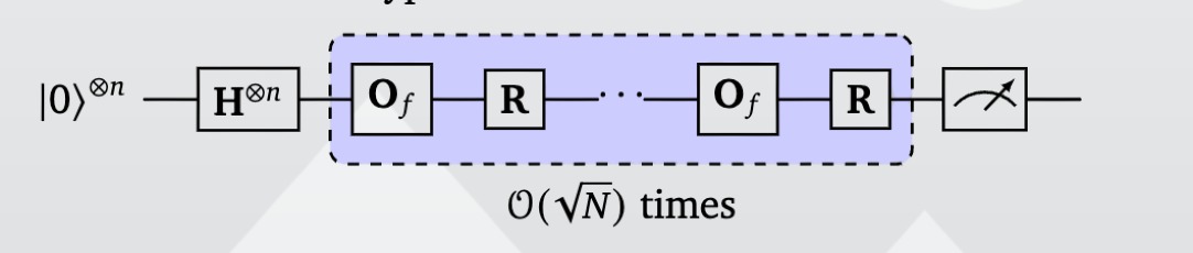
where $\mathbf{R}$ is the $n$-qubit unitary acting as

$$ \begin{align*} \ket{+}^{\otimes n} &\mapsto \ket{+}^{\otimes n} \\ \ket{\phi} &\mapsto - \ket{\phi} &&\text{ for all } \phi \perp \ket{+}^{\otimes n} \end{align*} $$

which describes a reflection about $\ket{+}^{\otimes n}$ or a uniform superposition over all $n$-bit strings. for those of us who like thinking of transformations as matrices; $\mathbf{R}$ can be explicitly written as the matrix $2 \ket{+}\bra{+}^{\otimes n} - \mathbb{I}$.

analysis

The time has now come to analyze the circuit for Grover’s algorithm. Let us assume for simplicity, that there is a single marked input $\mathbf{x^*} \in \{0, 1\}^n$. We start with $\ket{0}^{n}$ and prepare a uniform superposition by applying $\mathbf{H}^{\otimes n}$;

$$ \begin{align*} \ket{0}^n &\substack{\mathbf{H}^{\otimes n} \\ \mapsto} \frac{1}{\sqrt{N}} \sum_{x \in \{0, 1\}^n} := \ket{\psi} \end{align*} $$

For the sake of notational convenience, we will write the state $\ket{\psi}$ in terms of the marked input and the rest of the $n$-bit strings. This provides

$$ \begin{align*} \ket{\psi} &= \frac{1}{\sqrt{N}} \ket{x^*} + \frac{1}{\sqrt{N}} \sum_{x \neq x^*} \ket{x} = \frac{1}{\sqrt{N}} \ket{G} + \sqrt{\frac{N - 1}{N}} \ket{B} \end{align*} $$

where $\ket{G} := \ket{x^*}$ is the “good part” of the superposition and $\ket{B} := \frac{1}{\sqrt{N - 1}} \sum \limits_{x \neq x^*} \ket{x}$ is the “bad part” of the superposition; the part of the input that we don’t care about. Note that the normalization here is just so that $\ket{G}$ and $\ket{B}$ are valid quantum states.

Now given that this is a quantum algorithm, we have to make some kind of measurement towards the end. Were we to measure now, we would get the marked input $\mathbf{x}^*$ with very low probability, precisely $\frac{1}{N}$. At a high-level, our hope is to somehow “amplify” the amplitude of this coefficient so as to ensure we get the marked input string with very high probability when we measure. This is exactly what the Grover iterates or the repeated application of $\mathbf{O_f} \mathbf{R}$ achieves for us.

Before we dive into what the Grover iterate does for us, let us first massage our state into a more convenient expression. We write

$$\begin{align*} \ket{\psi} &= \frac{1}{\sqrt{2^n}} \ket{G} + \sqrt{\frac{2^n - 1}{2^n}} \ket{B} = \sin(\theta) \ket{G} + \cos(\theta) \ket{B} &&\text{ where } \sin(\theta) := \frac{1}{\sqrt{2^n}} \end{align*}$$

the effect of a single grover iterate

We first analyze the action of $\mathbf{R}$ on the states $\ket{G}, \ket{B}$.

$$\begin{align*} \mathbf{R} \ket{G} &= (2 \ket{+}\bra{+}^n - \mathbb{I}) \ket{x^*} \\ &= 2 \braket{+^n, x^*} \ket{+^n} - \ket{x^*} = \frac{2}{\sqrt{N}} \ket{+}^n - \ket{x^*} \\ &= \frac{2}{N} \sum_{x \in \{0, 1\}^n} \ket{x} - \ket{x^*} \\ &= \left(\frac{2}{N} - 1\right) \ket{G} + \frac{2 \sqrt{N - 1}}{N} \ket{B} \\ \mathbf{R} \ket{B} &= (2 \ket{+}\bra{+}^n - \mathbb{I}) \ket{B} \\ &= 2 \braket{+^n, B} \ket{+}^n - \ket{B} = 2 \sqrt{\frac{N - 1}{N}} \ket{+}^n - \ket{B} \\ &= \frac{2 \sqrt{N - 1}}{N} \left(\sum_{x \neq x^*} \ket{x} + \ket{x^*}\right) - \ket{B} \\ &= \frac{2 \sqrt{N - 1}}{N} \ket{G} + \left[\frac{2(N - 1)}{N} - 1\right] \ket{B} \\ &= \frac{2 \sqrt{N - 1}}{N} \ket{G} + \frac{N - 2}{N} \ket{B} \end{align*}$$

We are now ready to analyze the effect of a single grover iterate. We have that

$$ \begin{align*} \ket{\psi} &= \frac{1}{\sqrt{N}} \ket{G} + \sqrt{\frac{N - 1}{N}} \ket{B} \\ &\substack{\mathbf{O}_f \\ \mapsto} - \frac{1}{\sqrt{N}} \ket{G} + \sqrt{\frac{N - 1}{N}} \ket{B} \\ &\substack{\mathbf{R} \\ \mapsto} - \frac{1}{\sqrt{N}} \left(\frac{2 - N}{N} \ket{G} + \frac{2\sqrt{N - 1}}{N} \ket{B}\right) \\ &+ \sqrt{\frac{N - 1}{N}} \left(\frac{2 \sqrt{N - 1}}{N} \ket{G} + \frac{N - 2}{N} \ket{B}\right) \\ &= \left[\frac{N - 2}{N \sqrt{N}} + \frac{2 (N - 1)}{N \sqrt{N}}\right] \ket{G} + \left[\frac{(N - 2)\sqrt{N - 1}}{N \sqrt{N}} - \frac{2 \sqrt{N - 1}}{N \sqrt{N}}\right] \ket{B} \\ &= \frac{3N - 4}{N \sqrt{N}} \ket{G} + \frac{(N - 4)\sqrt{N - 1}}{N \sqrt{N}} \ket{B} \end{align*} $$

Now recall the triple-angle trig formulas. These are useful because with our prescribed instantiations of $\sin(\theta), \cos(\theta)$.

$$ \begin{align*} \sin(3 \theta) &= 3 \sin(\theta) - 4 \sin^3(\theta) = 3 \frac{1}{\sqrt{N}} - 4 \frac{1}{N \sqrt{N}} = \frac{3N - 4}{N \sqrt{N}} \\ \cos(3 \theta) &= 4 \cos^3(\theta) - 3 \cos(\theta) = 4 \frac{N - 1}{N} \sqrt{\frac{N - 1}{N}} - 3 \sqrt{\frac{N - 1}{N}} \\ &= \frac{(N - 4)\sqrt{N - 1}}{N \sqrt{N}} \end{align*} $$

Look familiar? Our state after one grover iterate, therefore becomes

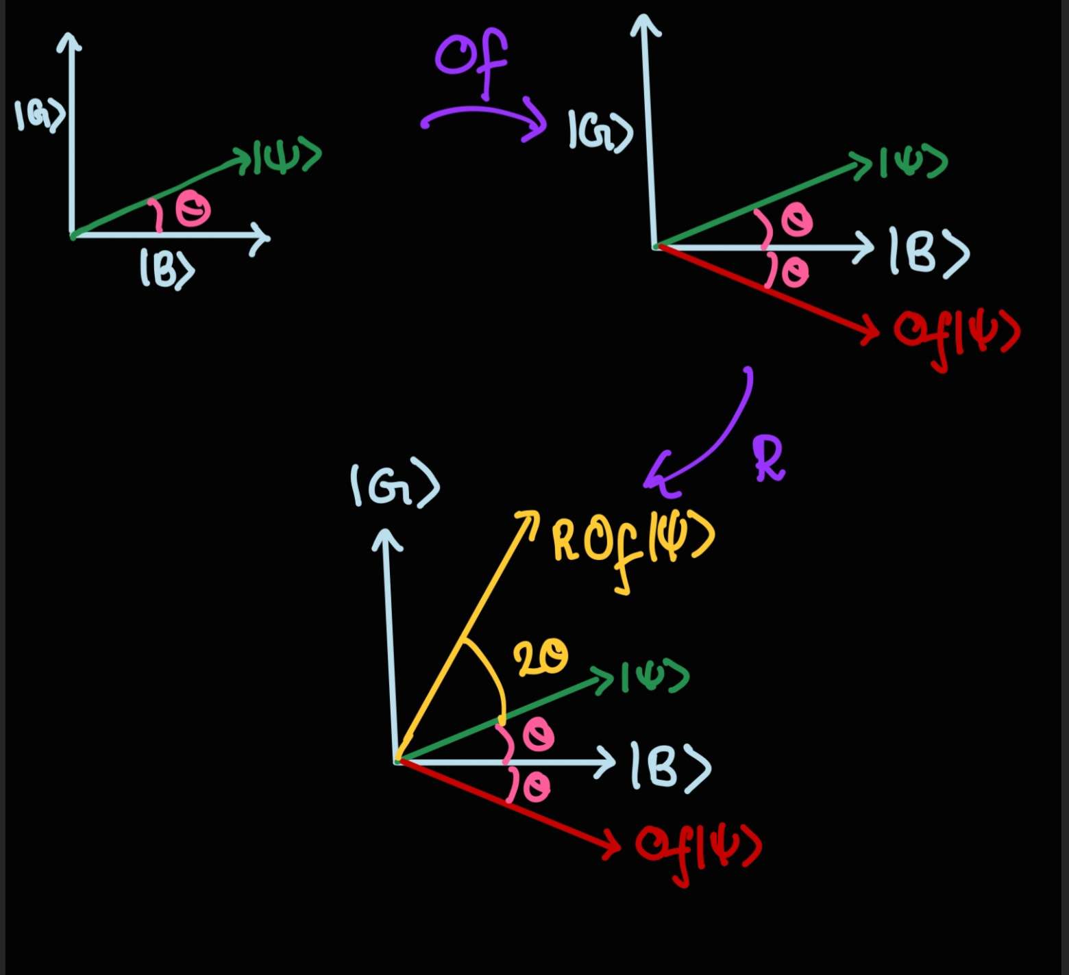
\[\begin{align*} \ket{\psi} &\substack{\mathbf{R} \mathbf{O}_f \\ \mapsto} \sin(3 \theta) \ket{G} + \cos(3 \theta) \ket{B} \end{align*}\]

Notice now that we started with a state $\ket{\psi} \in \text{span}\{\ket{G}, \ket{B}\}$ at an angle of $\theta$ with $\ket{B}$. After a single iterate, our state is now at an angle $3\theta$ with $\ket{B}$. From the above, we can also see that each application of $\mathbf{O}_f$ and $\mathbf{R}$ preserve the subspace $\text{span}\{\ket{G}, \ket{B}\}$. We started with a state in the span of $\ket{G}, \ket{B}$, and we end up with a state in the same space.

Therefore, each application of $\mathbf{R} \mathbf{O}_f$ rotates the state by an angle of $2 \theta$ towards $\ket{G}$. After $K$ grover iterates, the state becomes

\[\begin{align*} (\mathbf{R} \mathbf{O}_f)^K \ket{\psi} &= \sin((2K + 1) \theta) \ket{G} + \cos((2K + 1)\theta) \ket{B} \end{align*}\]

Geometrically one step of this entire process looks like the following.

success probability and # of iterations

In order to ensure high success probability (constant) when we measure the state in the $\ket{G}, \ket{B}$ basis, it suffices to pick $K$ such that $\sin((2K + 1) \theta)$ is large.

Invoking the small-angle sine approximation, we know that $\sin((2K + 1)\theta) \approx (2K + 1)\theta$ and picking $K = \mathcal{O}(\sqrt{N})$ is sufficient to find the marked input with constant probability.

what if we have multiple marked inputs?

In the setting where the number of marked inputs, i.e. $\mathbf{x}^* \in \{0, 1\}^n$ for which $f(\mathbf{x}^*) = 1$ is $\mathcal{L}$; we can follow a very similar procedure to the single marked input case. Define $\mathcal{S} := \{\mathbf{x}^* \in \{0, 1\}^n : f(\mathbf{x}^*) = 1\}$ to be the set of marked inputs.

We slightly alter the definitions of our “good states” and “bad states” respectively by putting

$$ \begin{align*} \ket{G} &:= \frac{1}{\sqrt{\mathcal{L}}} \sum_{x \in \mathcal{S}} \ket{x} \\ \ket{B} &:= \frac{1}{\sqrt{N - \mathcal{L}}} \sum_{x \notin \mathcal{S}} \ket{x} \end{align*} $$

The key difference here is that the initial angle $\theta$ is $\arcsin\left(\sqrt{\frac{\mathcal{L}}{N}}\right)$. By symmetric argument to the single marked input case, the overall runtime to acheive constant success probability is $\mathcal{O}\left(\sqrt{\frac{\mathcal{L}}{N}}\right)$.

references

footnotes

quantum channels ↩