the elevator pitch for quantum
today, we go distribution distinguishing
introduction
possibly the poster-child problem for an quantum computing class is the state discrimination problem. broadly speaking, the goal is to determine the unknown quantum state from a set of possible candidate states which are known to us as the distinguisher. note that this problem is trivial classically since given two classical states of information, one can always simply distinguish between them by simply reading the bits of which they are comprised. as the astute reader is well aware by now, such is not possible with quantum states; hence today’s post.
the problem itself
formally, the version of the state discrimination problem we will be dealing with is the following.
Given a pure \(d\)-dimensional state \(\ket{\psi}\in (\mathbb{C}^{2})^{\otimes d}\) known to be either \(\ket{\psi_1}\) or \(\ket{\psi_2}\), the goal is to output which state \(\ket{\psi}\) really is.
remark: there is a generalization of this problem where the distinguisher is handed a (possibly mixed) quantum state \(\rho \in \mathcal{L}(\mathbb{C}^{2^d})\) and is tasked with deciphering whether they were handed the state \(\rho_1\) or \(\rho_2\). it turns out that the classical analog of this problem is well-defined. in essence it equivocates to distinguishing between probability distributions \(\{p\}, \{q\}\) by drawing a single sample \(x\). further generalizations involve distinguishing between not just \(2\) states but rather a finite set of states \(\mathcal{S}\).
in order to quantify the performance of the strategies we come up with (natural or otherwise); for any algorithm $\mathcal{A}$, define how well it distinguishes two states $\ket{\psi_1}$ and $\ket{\psi_2}$ by
$$ \Delta(\mathcal{A}) := \frac{1}{2} \bigg[\Pr\left[\text{guess } \ket{\psi_1} \;\big|\; \ket{\psi_1}\right] + \Pr\left[\text{guess } \ket{\psi_2} \;\big|\; \ket{\psi_2}\right]\bigg] $$
where in words, \(\Delta\) quantifies our probability of success.
towards an optimal algorithm
what the naive strategy buys you
the most natural strategy is to measure in a basis for which \(\ket{\psi_1}\) is a basis element and guess “outcome \(1\)” if the measurement is \(\ket{\psi_2}\) otherwise. The success probability from this process via Born’s rule can be written as
$$ \begin{align*} \Delta(\mathcal{A}) &:= \frac{1}{2}\bigg[\left|\langle \psi_1 | \psi_1 \rangle\right|^2 + (1 - \left|\langle \psi_1 | \psi_2 \rangle\right|^2)\bigg] \\ &= 1 - \frac{1}{2}\left|\langle \psi_1 | \psi_2 \rangle\right|^2 \end{align*}
$$given the wording of the title of this section, it might not be surprising to most; that it is possible to do better.
a remark on the form of strategies we’re considering
I’ve been somewhat vague with the usage of the term “strategies” over here so before we dive into what the best one can hope for is, let us clarify the family of distinguishing strategies we are allowed to use. General strategies here are of the form
- Append some number of ancilla qubits to \(\ket{0}^n\)
- Apply a unitary \(\mathbf{U}\) to the joint system.
- Perform a two-outcome projective measurement \(\{\mathbf{P}, \mathbb{I} - \mathbf{P}\}\).
After sufficient amounts of meditation, one can show that steps \(2\) and \(3\) can be combined, i.e. the projective measurement we now perform is \(\{\mathbf{U}\mathbf{P}\mathbf{U}^\dagger, \mathbb{I} - \mathbf{U}\mathbf{P}\mathbf{U}^\dagger\}\). There is one more simplification we can make that is slightly more involved. It turns out that this entire process of appending ancillas and performing a projective-measurement is equivalent to performing a POVM. Therefore after all is said and done, the family of strategies we will be considering are of the form
- Perform “some” two-outcome POVM
an optimal algorithm
There exists a quantum strategy \(\mathcal{A}\) for which \(\Delta(\mathcal{A}) := \frac{1}{2} + \frac{1}{2}\sqrt{1 - |\braket{\psi_0|\psi_1}|^2}\)
proof: Our strategy \(\mathcal{A}\) is as follows. Let \(\ket{\mathbf{v}_0}, \ket{\mathbf{v}_1}\) be states in the span of \(\ket{\psi_0}, \ket{\psi_1}\) such that \(\langle \mathbf{v}_0 \mid \mathbf{v}_1 \rangle = 0\) and they are symmetric with respect to the angle bisector of \(\ket{\psi_0}\) and \(\ket{\psi_1}\) where \(\ket{\mathbf{v}_i}\) is closer to \(\ket{\psi_i}\). On outcome \(\ket{\mathbf{v}_i}\) we guess \(\ket{\psi_i}\). Illustratively, we have the following diagram.
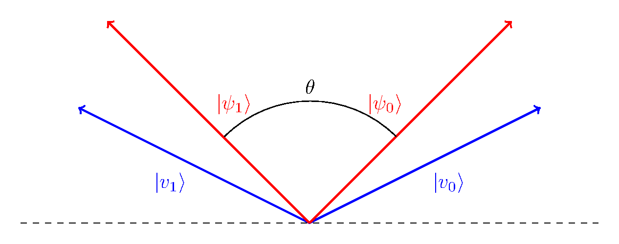
It now remains to compute \(\Delta\) for this strategy. Notice from the above description, that our strategy \(\mathcal{A}\) is symmetric with respect to \(\ket{\psi_1}\) and \(\ket{\psi_2}\). Therefore without loss of generality, we may assume \(\Delta = | \langle \mathbf{v}_1 \mid \psi_1 \rangle|^2\). Making use of the fact that the basis in which the measurement is made is orthonormal and the vectors \(\ket{\mathbf{v}_0}, \ket{\mathbf{v}_1}\) are completely real, one has
$$ \begin{align*} \Delta &= \left| \langle \mathbf{v}_1 \mid \psi_1 \rangle\right|^2 = \big|\braket{\psi_1|\mathbf{v}_1}\big|^2 = \|{\psi_0} \|^2 \|\mathbf{v}_0 \|^2 \cdot \cos(\angle (\psi_1, \mathbf{v}_1))^2 \\ &= \cos^2\left(\frac{\pi/2 - \theta}{2}\right) = \bigg| \frac{1}{2} + \frac{1}{2} \cos\left(\frac{\pi}{2} - \theta\right) \bigg|\\ &= \left|\frac{1}{2} + \frac{1}{2} \sin(\theta)\right| = \frac{1}{2} + \frac{1}{2}\sqrt{1 - |\braket{\psi_0|\psi_1}|^2} \end{align*} $$
remark: in this case, the POVM being applied is \(\{\vert \mathbf{v}\rangle \langle \mathbf{v}\vert, \mathbb{I} - \vert\mathbf{v}\rangle \langle \mathbf{v} \vert\}\) where \(\ket{\mathbf{v}}\) is the angle bisector between \(\ket{\psi_1}, \ket{\psi_2}\). Phrasing things here in terms of born’s rule instead of the POVM language is convenient since we’re dealing with pure states. However this generalization will be critical when we are dealing with mixed states (and shows up in demonstrating optimality)
generalizing to mixed states
As alluded to in the precursor of this text, we study the version of this problem where we are handed mixed states instead of pure ones. Recall the definition of a mixed state. A mixed state can be formally defined as a distribution over quantum states, i.e. \(\{p_i, \Phi_i\}_{i = 1}^n\) indicating that with probability \(p_i\), the state is given by \(\ket{\Phi_i}\). Mathematically, it can be represented by \(\rho = \sum \limits_{i = 1}^n p_i \vert \Phi_i \rangle \langle \Phi_i \vert\). As in the prior set-up, we are promised to receive \(\rho\) which is either \(\rho_1\) or \(\rho_2\) with equal probability. Before we analyze what the optimal quantum strategy looks like, let us answer this question classically so as to inform our intuition for quantum approaches.
At long last, the classical analogue
\(\mathcal{D}_1\) and \(\mathcal{D} _2 : [d] \to [0, 1]\) are two probability distributions and we receive one sample \(x \sim \{\mathcal{D}_1, \mathcal{D}_2\}\) and are tasked with identifying which distribution our sample came from. Classically strategies can be completely specified by functioons \(f : [d] \to \{\mathcal{D}_1, \mathcal{D}_2\}\) where in words \(f\) guides our guess of distribution when receiving some arbitrary sample.
An optimal classical strategy
Put \(p_i := \Pr \limits_{\mathcal{D}_1}[i]\), \(q_i := \Pr \limits_{\mathcal{D}_2}[i]\). Further define \(\mathcal{S} := \{i \in [d] : p_i \geq q_i\}\). The optimal strategy is now upon receiving some arbitrary sample \(j \sim \{\mathcal{D}_1, \mathcal{D}_2\}\). If \(j \in \mathcal{S}\), guess \(\mathcal{D}_1\). Otherwise guess \(\mathcal{D}_2\). Similar to above, we compute \(\Delta\) for this strategy. Let \(j\) be our sample. Then, we have that
$$ \begin{align*} \Delta(\mathcal{A}) &= \frac{1}{2} \bigg[\Pr[\text{guess } \mathcal{D}_1 \mid \mathcal{D}_1] + \Pr[\text{guess } \mathcal{D}_2 \mid \mathcal{D}_2]\bigg] \\ &= \frac{1}{2} \bigg[\Pr[\text{guess } \mathcal{D}_1 \mid \mathcal{D}_1] + 1 - \Pr[\text{guess } \mathcal{D}_1 \mid \mathcal{D}_2]\bigg] \\ &= \frac{1}{2} + \frac{1}{2} \bigg[\Pr[j \in \mathcal{S} \mid j \sim \mathcal{D}_1] - \Pr[j \in \mathcal{S} \mid j \sim \mathcal{D}_2]\bigg] \\ &= \frac{1}{2} + \frac{1}{2} \sum_{i \in \mathcal{S}} p_i - q_i = \frac{1}{2} + \frac{1}{2} \vert \vert \mathcal{D}_1 - \mathcal{D}_2 \vert \vert_{\text{TV}} \end{align*}$$
where the second equality in the last line comes from our choice of \(\mathcal{S}\) and the norm in question is referring to the total variation distance between two probability measures.
an argument for (classical) optimality
Based on our above computation, optimality follows immediately. Inspired by our definition of classical strategies, put \(S := \{i : f(i) \in \mathcal{D}_1\}\). Then to a calculation similar as the above; we obtain
$$ \begin{align*} \Delta &= \frac{1}{2} \bigg[\Pr[\text{guess } \mathcal{D}_1 \mid \mathcal{D}_1] + \Pr[\text{guess } \mathcal{D}_2 \mid \mathcal{D}_2]\bigg] \\ &= \frac{1}{2} \bigg[\sum_{i \in S} p_i + \sum_{i \notin S} q_i\bigg] = \frac{1}{2} + \frac{1}{2} \bigg[\sum_{i \in S} p_i - q_i\bigg] \end{align*} $$
and so the above problem now reduces to choosing \(S \subseteq [d]\) in order to maximize \(\sum \limits_{i \in S} (p_i - q_i)\). This is friendly since the maximizing \(S^*\) is given by
$$ \begin{align*} S^* = \{i \in [d] : p_i - q_i \geq 0\} = \{i \in [d] : p_i \geq q_i\} \end{align*} $$
This completes the proof.
an argument for (quantum) optimality
The arrangement of things here is slightly strange since we haven’t explicitly argued a strategy for distinguishing between two mixed states, but it may help to first see what the maximum likelihood of success is for a general quantum strategy and construct a measurement procedure (POVM) in order to acheive this. Recall form three of our quantum strategy. We may therefore assume without loss of generality that our quantum strategy consists of a two-outcome POVM \(\{\Pi_1, \Pi_1\}\) that that when we measure outcome \(1\), we guess \(\rho_1\) and otherwise we guess \(\rho_2\). The probability of success is thereby
$$ \begin{align*} \Delta &= \frac{1}{2} \bigg\{\Pr[\text{guess } \rho_1 \mid \rho_1 ] + \Pr[\text{guess } \rho_2 \mid \rho_2 ]\bigg\} \\ &= \frac{1}{2} + \frac{1}{2} \bigg\{\Pr[\text{guess } \rho_1 \mid \rho_1 ] - \Pr[\text{guess } \rho_1 \mid \rho_2 ]\bigg\} \\ &= \frac{1}{2} + \frac{1}{2} \left\{\text{Tr}(\Pi_1 \rho_1) - \text{Tr}(\Pi_1 \rho_2)\right\} \\ &= \frac{1}{2} + \frac{1}{2} \text{Tr} [\Pi_1(\rho_1 - \rho_2)] \end{align*} $$
and so therefore the guessing probability is given by
$$ \begin{align*} \textsf{OPT} := \max_{\mathbf{0} \preceq \Pi_1 \preceq \mathbb{I}} \bigg[\frac{1}{2} + \frac{1}{2} \text{Tr} [\Pi_1(\rho_1 - \rho_2)]\bigg] \end{align*} $$
The game is now completely governed by picking an appropriate \(\Pi_1\). Now, since \(\rho_1 - \rho_2\) is Hermitian, by the spectral theorem we can write \(\rho_1 - \rho_2 = \sum \limits_{i} \lambda_i \vert v_i \rangle \langle v_i \vert\) where \(\{\vert v_1 \rangle, \ldots, \vert v_n\rangle\}\) is the shared eigenbasis and \(\lambda_i\) are the corresponding eigenvalues. This then provides
$$ \begin{align*} \text{Tr}[\Pi_1 (\rho_1 - \rho_2)] &= \sum_{i} \lambda_i \text{Tr}[\Pi_1 \vert v_i \rangle \langle v_i \vert] = \sum_i \lambda_i \underbrace{\langle v_i \vert \Pi_1 \vert v_i \rangle}_{\in [0, 1]} \\ &\leq \sum_{i : \lambda_i \geq 0} \lambda_i \end{align*} $$
It now remains to argue that this upper bound can actually be acheived. Indeed picking \(\Pi_1 := \sum \limits_{i : \lambda_i \geq 0} \lambda_i \vert v_i \rangle \langle v_i \vert\) suffices to achieve the optimal value (It can also be verified that this is a valid choice of POVM).
An outline of the optimal quantum strategy
After all is said and done, we can now outline the quantum strategy that is the object of today’s study. Let \(\{\vert v_1 \rangle, \ldots, \vert v_n \rangle\}\) be an eigenbasis of \(\rho_1 - \rho_2\) with correponding eigenvalues \(\{\lambda_1, \ldots, \lambda_n\}\). Put \(S := \{i \in [d] : \lambda_i \geq 0\}\). The optimal strategy is on receiving \(\rho\) to measure the state in the aforementioned eigenbasis and upon receiving outcome \(i\), guess \(\rho_1\) iff \(i \in S\). Otherwise guess \(\rho_2\).
A final connection to the trace distance
The optimal success probability from our exposition above is given by
$$ \begin{align*} \Delta_{\textsf{OPT}} &= \frac{1}{2} + \frac{1}{2} \sum_{i : \lambda_i \geq 0} \lambda_i = \frac{1}{2} + \frac{1}{4} \sum_{i} |\lambda_i| \\ &= \frac{1}{2} + \frac{1}{4} \vert \vert \rho_1 - \rho_2 \vert \vert_{1} = \frac{1}{2} + \frac{1}{2} \vert \vert \rho_1 - \rho_2 \vert \vert_{\text{tr}} \end{align*} $$
where the second equality in the first line follows from \(\text{Tr}(\rho_1 - \rho_2) = 0\) and the norms in question are the sum of the singular values of \(\rho_1 - \rho_2\) and \(\vert \vert \cdot \vert \vert_{\text{tr}}\) is defined to be the trace distance and is equal to half the “\(\ell_1\)-distance”. This is also why sometimes the trace distance is sometimes defined as the maximum distingushing probability between two states, i.e.
$$ \begin{align*} \vert \vert \rho - \sigma \vert \vert_{\text{tr}} &= \sup_{\mathbf{0} \preceq \Pi \preceq \mathbb{I}} \text{Tr}[\Pi(\rho - \sigma)] \end{align*} $$