so i gave a theory talk

the petersen graph is in almost every sense of the word; a universal counter-example

notation and some motivation

notation:

Before I get to some of the really cool motivation for this problem, I wanna make sure that everyone here is familiar with the the kinds of graphs we’ll be working with in the domain of this proof.

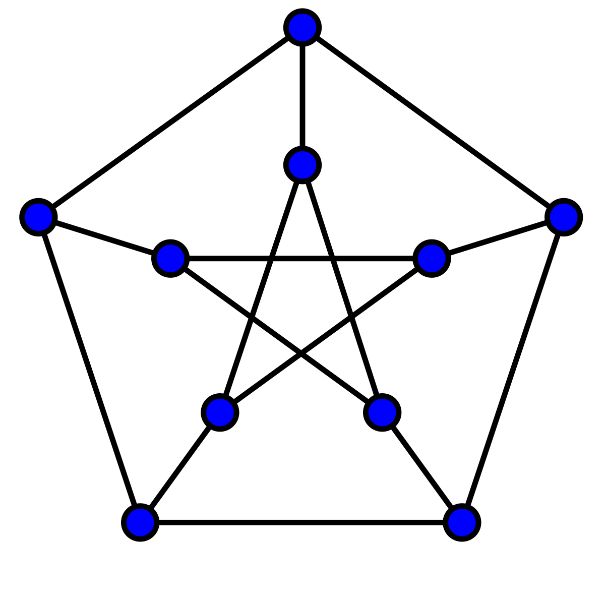
This is the Petersen graph. Veteran graph theoreticians will be familiar with this pentagram inscribed within the spokes of a regular pentagon. The Petersen graph is used as a counter example in tons of graph theory proofs which is one of the reasons it’s so well studied, partly what we’ll be doing here. The Petersen graph has $10$ nodes and $15$ edges, and is what we call $3$-regular.

Note: A graph is said to be $d$-regular iff every vertex has the same degree $d$. (i.e. it is strongly regular)

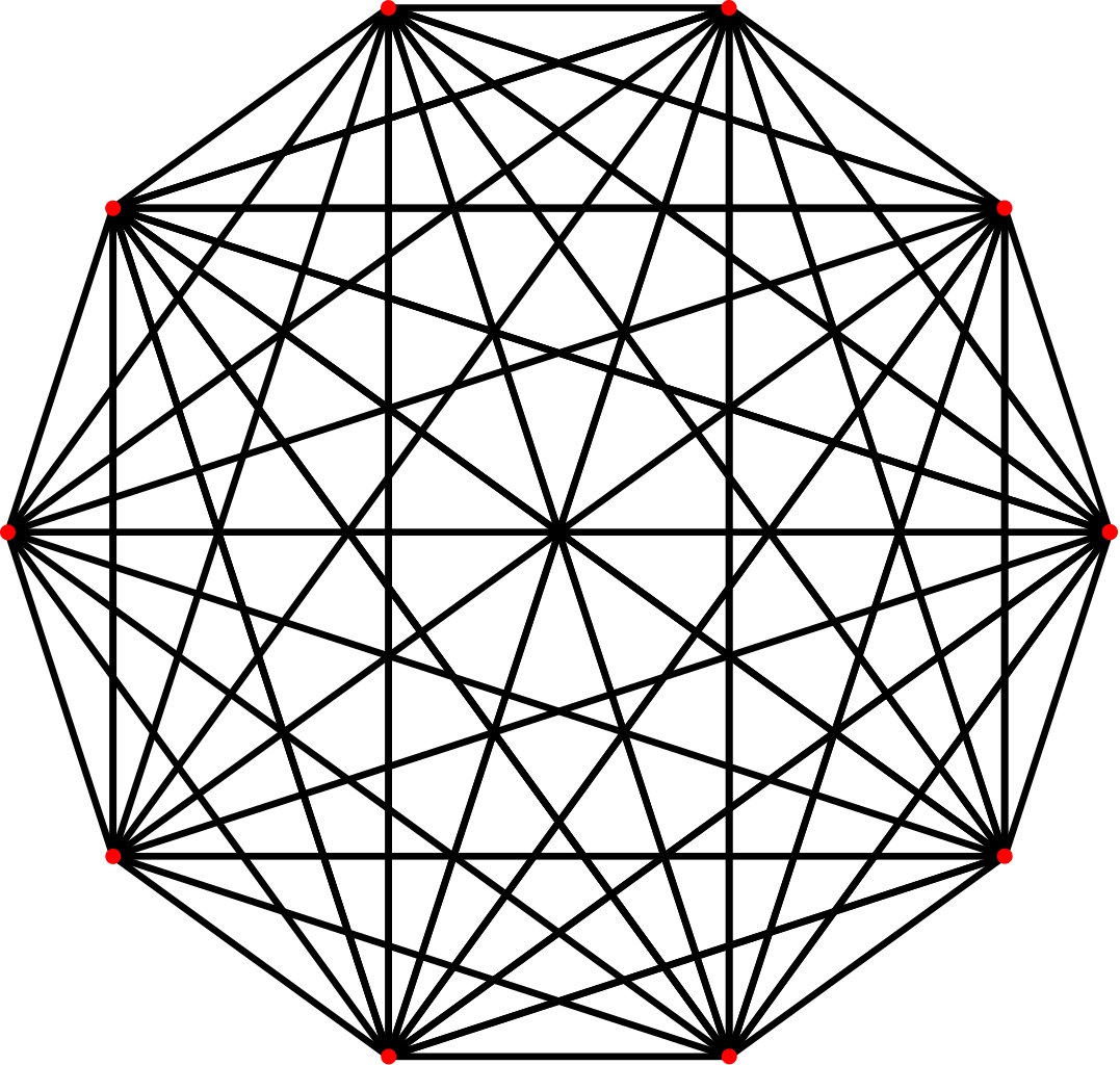
This is the complete graph on $10$ vertices. For the sake of convenience, we will refer to this graph as $K_{10}$. It has $10$ nodes and $45$ edges (i.e., all possible edges among $10$ nodes). If we follow along from the same scheme of defining things, the number of edges in $K_{n}$ (the complete graph with $n$ vertices) is given by $\binom{n}{2}$.

In this proof, $\mathbf{J}_{n}$ refers to the all ones matrix with dimension/size $n \times n$.

The row space of a matrix $\mathbf{A}$ is defined as follows, $\text{Row}(A) = \\{\mathbf{y}^{\mathbf{\top}} A : \mathbf{y} \in \mathbb{R}^{n}\\}$

definition

$$ \textsf{Trace}(\mathbf{A}) = \sum \limits_{x \in E_{x}(\mathbf{A})} \lambda_{x} $$

lemma 1

For a symmetric matrix $\mathbf{A}$, eigenvectors corresponding to distinct eigenvalues are orthogonal

proof
Let $\mathbf{x}$ and $\mathbf{y}$ be eigenvectors of the matrix $\mathbf{A}$ corresponding to eigenvalues $\lambda_1$ and $\lambda_2$ respectively. Therefore we have that

$$ \begin{align*} \mathbf{y}^{\top} \mathbf{Ax} = \mathbf{y}^{\top} \lambda_1 \mathbf{x} &\implies \mathbf{y}^{\top} \mathbf{A}^\top \mathbf{x} = \mathbf{y}^{\top} \lambda_1 \mathbf{x} \\ &\implies \mathbf{(Ay)}^{\top} \mathbf{x} = \lambda_1 \mathbf{y}^{\top}\mathbf{x} \\ &\implies (\lambda_2 \mathbf{y})^\top \mathbf{x} = \lambda_2 \mathbf{y}^{\top}\mathbf{x} \\ &\implies \mathbf{y}^{\top}\mathbf{x} (\lambda_2 - \lambda_1) = 0 \end{align*} $$

However, we already know that $\lambda_2 \neq \lambda_1$. Therefore $\lambda_2 - \lambda_1 \neq 0$, and it must be the case that $\mathbf{y}^{\top}\mathbf{x} = 0$.

Therefore $x$ and $y$ are orthogonal.

adjacency matrices:

definition

We define the adjacency matrix of a graph $G = (V, E)$ as the following,

$$ A_{ij} = \begin{cases}1 & \text{there is an edge from} \; j \; \text{to} \; i\\0 & \text{there is no edge from} \; j \; \text{to} \; i\\ \end{cases} $$

Since we’re dealing with an undirected graph in this proof, every edge $(a, b)$ is counted as the same edge as if there were an edge $(b, a)$ in the graph. As a consequence, the adjacency matrices for this family of graphs will be symmetric.

The way to think about it is that the adjacency matrix of a graph $G$ encodes information about the number of length $1$ paths between any pair of vertices $i$ and $j$, i.e. information about the vertices immediately “adjacent” to each other.

motivation:

Each node in $K_{10}$ has $9$ edges incident to it while each node in the Petersen graph has $3$ edges incident to it. So it is plausible that $K_{10}$ can be covered perfectly by $3$ Petersen graphs. This means that you can lay down three Petersens on $K_{10}$ so that vertices go to vertices and each edge of $K_{10}$ lies under an edge of exactly one of the three Petersens. This hints at some pretty cutting-edge stuff in the field of graph decomposition and graph coloring and the parallels in higher dimensions is absolutely incredible. With some linear algebra at our disposal, we will show that it is not possible to completely cover $K_{10}$ with three Petersen graphs.

eigenvalues of the petersen graph

Finding the eigenvalues of any matrix, let alone one that of size $10 \times 10$ is a fairly computational task and isn’t enlightening in any form whatsoever. So why are we trying to find the eigenvalues of the petersen graph? Well we can take advantage of the fact that the adjacency matrix represents information that carries physical meaning (vertex-edge relations of a graph) and can use the language of linear transformations and some geometric intuition to gain insight into the eigenvalues of this graph.

Let $\mathbf{A}$ be the adjacency matrix of the Petersen Graph. If $\mathbf{A}$ encodes information about the number of length $1$, $\mathbf{A}^2$ represents information about the number of length $2$ paths, and in general, $A^k$ encodes information about the number of $k$-length paths in a given graph. With this information in our belt, we know can make a pretty nifty observation.

Consider the $i, j^{th}$ entry of the matrix $\mathbf{A}^2 + \mathbf{A}$ (the sum of the matrices representing information about the number of length $2$ paths and the regular adjacency matrix of the petersen graph). Since, every vertex in the petersen graph has degree $3$, each vertex has $3$ length $2$ paths back itself whereas there are no length $1$ paths from a vertex to itself. With this information under our belt, we can say that

$$ (A^2 + A)_{ij} = \begin{cases} 3 & \forall i = j \\ 1 & \forall i \neq j \end{cases} $$

This follows from noticing that any pair of vertices not already joined by an edge are joined by a unique path of length $2$; namely there is a unique vertex which is joined to both.

We can therefore conclude that the matrix $\mathbf{}$ satisfies the matrix equation $\mathbf{A}^2 + \mathbf{A} = 2\mathbf{I} + \mathbf{J}$

Note that $\mathbf{J}$ has eigenvalue 10 (of multiplicity 1 with eigenvector 1) and eigenvalue 0 of multiplicity 9. Thus $2\mathbf{I} + \mathbf{J}$ has eigenvalue 12 of multiplicity 1 and eigenvalue 2 of multiplicity 9. Now if $x$ is an eigenvector of A of eigenvalue $\lambda$ then $\mathbf{x}$ is an eigenvector of $\mathbf{A}^2 + \mathbf{A}$ of eigenvalue $\lambda^2 + \lambda$.

Thus the possible eigenvectors for $\mathbf{A}$ are prescribed. We already know that $\mathbf{1}$ is an eigenvector of $\mathbf{A}$ of eigenvalue 3 (or at least it is easy to check). The other 9 eigenvalues must satisfy $\lambda^2 + \lambda = 2$ thus either 1 or -2 with total multiplicity being 9. Now the trace of $\mathbf{A}$, which is 0, is the sum of the eigenvalues and so we deduce that 1 has multiplicity 5 and -2 has multiplicity 4.

the actual proof

lemma 2

If $\mathbf{K}_{10}$ represents the adjaceny matrix of the complete graph on 10 vertices, $\mathbf{J}_{10}$ represents the matrix with all its entries being equal to $1$ and $\mathbf{I}_{10}$ represents the identity matrix of size $10 \times 10$, then

$$ \begin{align*}\mathbf{K}_{10} = \mathbf{J}_{10} - \mathbf{I}_{10}\end{align*} $$

proof: The adjacency matrix of $K_{10}$ has all but its diagonal entries being equal to $1$, since every node in the full graph is connected to every other node except itself. The diagonal entries of $\mathbf{K}_{10}$ are filled in with $0$’s since there is no path from any of the nodes to itself. One can also clearly see that the matrix described by the equation $\mathbf{J}_{10} - \mathbf{I}_{10}$ is a matrix that has all but its diagonal entries being equal to $1$ and its diagonal entries being equal to $0$.

Therefore the adjacency matrix of $\mathbf{K}_{10} = \mathbf{J}_{10} - \mathbf{I}_{10}$

Assumption:

$$ \begin{align*}\mathbf{A}_P + \mathbf{A}_Q + \mathbf{A}_R = J_{10} - I_{10}\end{align*} $$

We consider three permutation matrices of the Petersen Graph $A_P, A_Q$ and $A_R$ (matrices formed by simultaneous row and column swaps in the original adjacency matrix of the petersen graph). We construct each of these permutation matrices such that $A_Q = CAC^{-1}$ where $C$ is some matrix. By this construction, $A_Q$ and $A$ are similar, and an important consequence is that they have the same eigenvalues. This assumption and construction is true for $A_P$ and $A_R$.

lemma 3

$$ \text{Null} (\mathbf{A}_P - \mathbf{I}_{10}) \subseteq \text{Span} (\mathbf{1})^{\perp} $$

proof: We wish to show that $\mathbf{1}^{\top} = \mathbf{y}^{\top}(\mathbf{A}_P - I_{10})$ for some vector $\mathbf{y} \in R^{10}$. Consider $\mathbf{y} = \mathbf{1}^{\top}$. The matrix product $\mathbf{1}^{\top}(\mathbf{A}_P - \mathbf{I}_{10})$ yields the vector whose entries are the sum of the entries of the columns of $\mathbf{A}_P - \mathbf{I}_{10}$. for an arbitrary column $i$ in its adjacency matrix, by the way the Petersen graph was defined we know that he graph has 3 outgoing edges which means that the sum of the entries of a column in its adjacency matrix is 3. However note that the diagonal entries of the adjacency matrix will be 0 since the Petersen graph does not contain self-loops. After subtracting the $i$th column of $\mathbf{I}_{10}$, the sum of the columns of the matrix $\mathbf{A}_P - \mathbf{I}_{10}$ is 2. Note that the identity matrix has 0 in every entry where $i \neq j$. Since the above holds true for an arbitrary column of the matrix, We can conclude that every column of $\mathbf{A}_P - \mathbf{I}_{10}$ sums up to a 2. More fundamentally, the product $\mathbf{1}^{\top}(\mathbf{A}_{P} - \mathbf{I}_{10})$ generates the all twos vector or 2$\mathbf{1}^{\top}$.

Therefore we can assert that $\text{Span}(\mathbf{1}) \subseteq \text{Row} (\mathbf{A}_P - \mathbf{I}_{10})$.

side proof

Let $A$ and $B$ be two subspaces such that $A \subseteq B$, then

$$ B^{\perp} \subseteq A^{\perp} $$

proof Let $\mathbf{x} \in B^{\perp}$. By definition of the orthogonal complement, we have that $\forall \mathbf{v} \in B, \mathbf{x}^{\top}\mathbf{v} = 0$. However we know that any vector contained in $B$ will be a vector contained in $A$, ($A$ is a subset of the vectors contained in $B$). Therefore $\mathbf{x}$ is orthogonal to every vector in $A$. By definition, this means that $\mathbf{x} \in A^{\perp}$ $\therefore A \subseteq B \implies B^{\perp} \subseteq A^{\perp}$

Using the aforementioned proof and taking orthogonal complements, we have that

$$ \begin{align*} \text{Span}(\mathbf{1}) \subseteq \text{Row} (\mathbf{A}_P - \mathbf{I}_{10}) &\implies \text{Null} (\mathbf{A}_P - \mathbf{I}_{10}) \subseteq \text{Span} (\mathbf{1})^{\perp} \\ &\implies \text{Null} (\mathbf{A}_P - \mathbf{I}_{10}) \subseteq \text{Span} (\mathbf{1})^{\perp} \end{align*} $$

The above results are also true for $\mathbf{A}_Q - \mathbf{I}_{10}$ since $Q$ is also a Petersen graph.

lemma 4

Assuming the standard definitions of the matrices $A_P, A_Q$ and $A_R$, we have that

$$ \text{Null} (\mathbf{A}_P - \mathbf{I}_{10}) \cap \text{Null} (\mathbf{A}_Q - \mathbf{I}_{10}) \neq \{0\} $$

proof For two subspaces $R_1$ and $R_2$ of $\mathbb{R}^{9}$, if $S_1 \cap S_2 = \{0\}$, then $B_{S_1}$ and $B_{S_2}$ are linearly independent. We therefore prove by contrapositive.

We also know that

$$ \text{Null} (\mathbf{A}_P - \mathbf{I}_{10}) \subseteq \text{Span} (\mathbf{1})^{\perp} \quad \text{and} \quad \text{Null} (\mathbf{A}_Q - \mathbf{I}_{10}) \subseteq \text{Span} (\mathbf{1})^{\perp} $$

$B_{\text{Null} (\mathbf{A}_P - \mathbf{I}_{10})} \cup B_{\text{Null} (\mathbf{A}_Q - \mathbf{I}_{10})}$ has 10 vectors in $\mathbb{R}^{9}$ since the bases of each of the null spaces has 5 vectors. Therefore $B_{\text{Null} (\mathbf{A}_P - \mathbf{I}_{10})} \cup B_{\text{Null} (\mathbf{A}_Q - \mathbf{I}_{10})}$ must be linearly dependent (since they have more vectors than the dimension of the space they exist in).

Therefore $B_{S_1} \cap B_{S_2} \neq \{0\}$ where $S_1$ and $S_2$ refer to the two subspaces above. This implies the existence of a non-zero vector $w$ that exists in their intersection.

The larger consequence of this is that this vector $\mathbf{w}$ is orthogonal to the all ones vector, i.e. ${\bf 1}^{\top} \mathbf{w} = 0$

the final stages

$$ \begin{align*} \mathbf{A}_P(\mathbf{v}) &= \lambda \mathbf{v} = \mathbf{v} &&\text{Since 1 is an eigenvalue of $$\mathbf{A}_P$$} \\ \mathbf{A}_R(\mathbf{w}) &= \mathbf{J}_{10}(\mathbf{w}) - \mathbf{I}_{10} (\mathbf{w}) - \mathbf{A}_P(\mathbf{w}) - \mathbf{A}_Q(\mathbf{w}) \\ &= \mathbf{J}_{10}(\mathbf{w}) - \mathbf{w} - \mathbf{w} - \mathbf{w} \end{align*} $$

We now compute $J_{10} (w)$ where $w \in \text{Null} (A_P - I_{10})$

$$ \mathbf{J}_{10}\mathbf{w} = \begin{bmatrix} 1 & 1 & 1 & 1 & 1 & 1 & 1 & 1 & 1 & 1 \\ 1 & 1 & 1 & 1 & 1 & 1 & 1 & 1 & 1 & 1 \\ 1 & 1 & 1 & 1 & 1 & 1 & 1 & 1 & 1 & 1 \\ 1 & 1 & 1 & 1 & 1 & 1 & 1 & 1 & 1 & 1 \\ 1 & 1 & 1 & 1 & 1 & 1 & 1 & 1 & 1 & 1 \\ 1 & 1 & 1 & 1 & 1 & 1 & 1 & 1 & 1 & 1 \\ 1 & 1 & 1 & 1 & 1 & 1 & 1 & 1 & 1 & 1 \\ 1 & 1 & 1 & 1 & 1 & 1 & 1 & 1 & 1 & 1 \\ 1 & 1 & 1 & 1 & 1 & 1 & 1 & 1 & 1 & 1 \\ 1 & 1 & 1 & 1 & 1 & 1 & 1 & 1 & 1 & 1 \end{bmatrix} \mathbf{w} = \begin{bmatrix} \mathbf{1}^{\top} \\ \mathbf{1}^{\top} \\ \mathbf{1}^{\top} \\ \mathbf{1}^{\top} \\ \mathbf{1}^{\top} \\ \mathbf{1}^{\top} \\ \mathbf{1}^{\top} \\ \mathbf{1}^{\top} \\ \mathbf{1}^{\top} \\ \mathbf{1}^{\top} \end{bmatrix}w = \begin{bmatrix} \mathbf{1}^{\top} \mathbf{w} \\ \mathbf{1}^{\top} \mathbf{w} \\ \mathbf{1}^{\top} \mathbf{w} \\ \mathbf{1}^{\top} \mathbf{w} \\ \mathbf{1}^{\top} \mathbf{w} \\ \mathbf{1}^{\top} \mathbf{w} \\ \mathbf{1}^{\top} \mathbf{w} \\ \mathbf{1}^{\top} \mathbf{w} \\ \mathbf{1}^{\top} \mathbf{w} \\ \mathbf{1}^{\top} \mathbf{w} \end{bmatrix} = \begin{bmatrix} 0 \\ 0 \\ 0 \\ 0 \\ 0 \\ 0 \\ 0 \\ 0 \\ 0 \\ 0 \end{bmatrix} $$

\[\therefore \mathbf{A}_R(\mathbf{w}) = \mathbf{J}_{10}(\mathbf{w}) - \mathbf{w} - \mathbf{w} - \mathbf{w} = -3\mathbf{w}.\]

We have therefore arrived at a contradiction. In the beginning of the proof, we found all the eigenvalues of the Petersen Graph and concluded that -3 was not amongst that list. However as we can see, we have proved that -3 in fact is an eigenvalue for the adjacency matrix of a Petersen graph. Therefore it is not possible to cover the full graph or $K_{10}$ with 3 Petersen graphs.

key takeaways

How cool is this!! All we did here was take advantage of some fairly simple linear algebra to prove a really fundamental fact about graphs that pop up quite frequently in the study of networks. For those interested, there is a conjecture in the “colorful” field of graph decomposition by the name of Ringel’s Conjecture that actually illustrates how exactly you can cover complete graphs of this variety. If there’s anything I want you to take away from this proof, it’s that geometric intution is unparalleled and this technique of analyzing eigenvalues not only can save you computation, it gives you critical insight into what the graph actually represents, a deeper understanding of what it “does”, so to speak. It is so easy to get bogged down in what might just seem like computation after computation. But there is a bigger picture, and that bigger picture is usually a bigger graph.

higher dimensions and moore graphs

degree-diameter problem: In graph theory, the degree diameter problem is the problem of finding the largest possible graph $G$ (in terms of the size of its vertex set $V$) of diameter $d$ such that the largest degree of the vertices in $G$ is at most $k$. The size of $G$ is bounded above by the Moore bound; In general, the largest degree-diameter graphs are much smaller than as prescribed by the Moore bound.

the moore bound and moore graphs The moore bound gives us an upper bound on how many nodes a graph can contain with diameter $d$ and maximum degree $k$. An intuitive way to recognize what the moore bound actually tells us is how wide a graph can get. Let $M$ be the moore bound that a graph of the above specifications can meet, we therefore have that

\[M = 1 + k \sum_{i = 0}^{d - 1} (k - 1)^i\]

Graphs that attain this bound $M$ are known as Moore graphs.

obtaining the moore bound

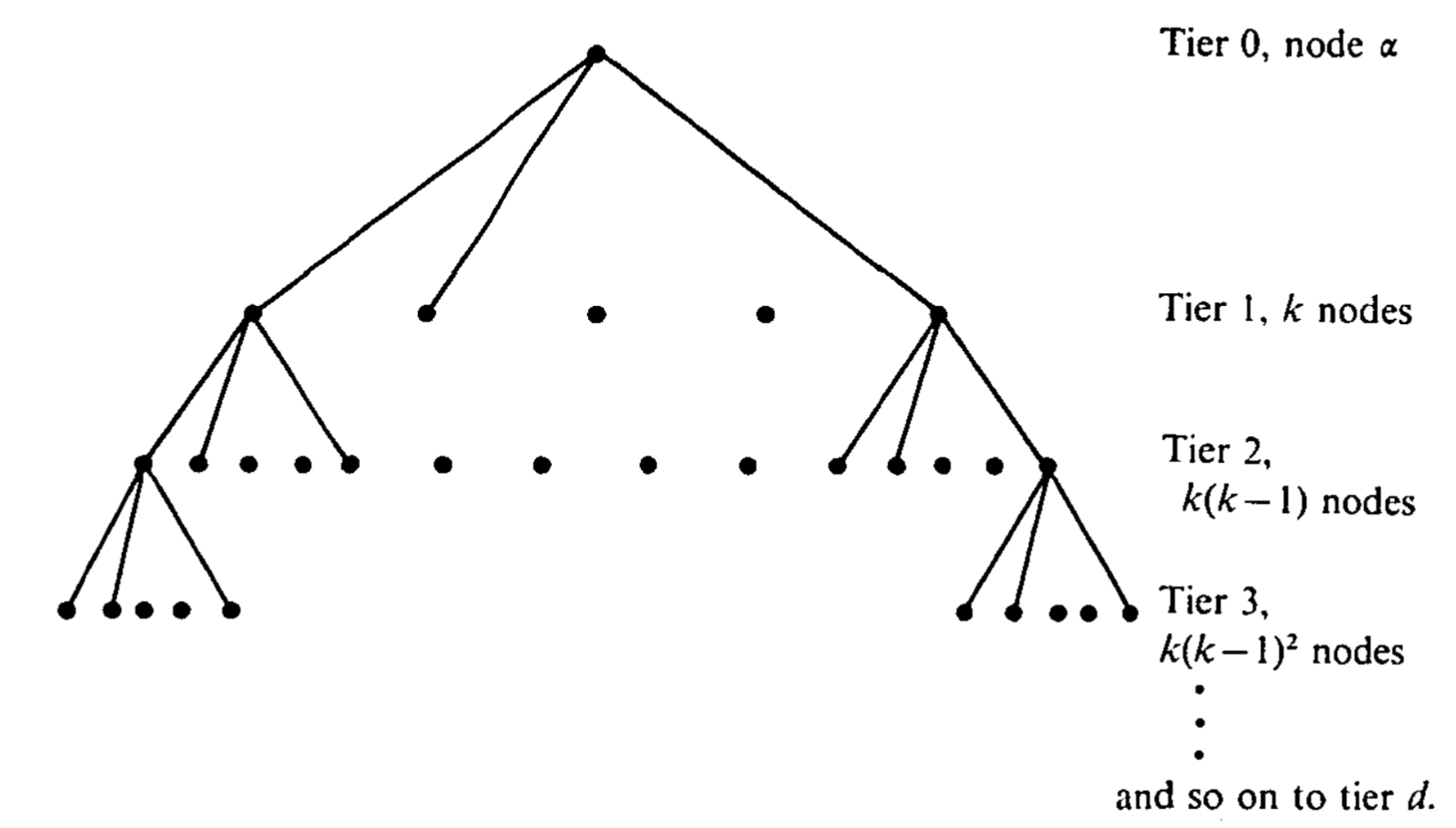
Consider the breadth first search of a graph $G$. From the above picture, we can clearly see that level 0 has only one node, this being the root of the tree generated by breadth first search. Level 1 has at most $k$ nodes since the maximum degree of any node in the graph is given by $k$. For each node $i$ in Level 1, $i$ can be connected to at most $k - 1$ nodes (it’s important not to forget the node they are connected to in Level 0). Since there are $k$ nodes in the first level, the maximum number of nodes in level 2 is given by $k(k - 1)$.

Generalizing, we have that the number of nodes in a level $j$ $\leq k(k - 1)^{j - 1}$.

Notice that we can count the nodes from level 1 to $d$ (we can’t have more than $d$ levels) using a sum given by $\sum_{i = 1}^{d} k(k - 1)^{i - 1}$. We also have to account for the root node which adds 1 to this total sum formula. After some substitution of variables, we get that the final expression for the upper bound comes out to be

\[M = 1 + k \sum_{i = 0}^{d - 1} (k - 1)^{i - 1}\]

types of moore graphs and its relation to the petersen graph The entire reason we’re even talking about moore graphs is that the petersen graph is a very specific kind of moore graph. Remember that equation we found for the adjacency matrix of the petersen graph. Well for the moore graphs that are known to exist, they satisfy the same “general form” of that equation.

lemma 5

The only $d$-regular Moore graphs of girth 5 and diameter 2 exist for $d = 2, 3, 7$ and possibly $57$.

proof Assume $G$ is a $d$-regular Moore graph of girth 5. A reminder that the girth of a graph is defined to be $2k + 1$ where $k$ is the diameter of the graph. Solving the above equation for the girth, we get that the diameter of the graph must be 2, i.e. $k = 2$. Substituting in this value into the Moore bound, we get that the number of the vertices in the graph is given by

\[n = 1 + d + d(d- 1) = d^{2} + 1\]

As we did for the petersen graph, we consider the square of the adjacency matrix $A^{2}$ once again. Notice that the adjacenct vertices don’t share any neighbours since if they did, there would be a triangle in $G$. Non-adjacent vertices share exactly one neighbor, because the diameter of $G$ is 2. Hence, $A^{2}$ has $d$ on the diagonal, 0 for edges and 1 for non-edges.

In other words, we have that

$$ (A^{2} + A)_{i, j} = \begin{cases} d & \forall i = j \\ 1 & \forall i \neq j \end{cases} $$

We therefore have that $\mathbf{A}$ satisfies the equation $\mathbf{A}^{2} + \mathbf{A} = (d - 1)\mathbf{I} + \mathbf{J}$

lemma 6

If $\lambda$ is an eigenvalue of $A$ different from $d$, we get from the above equation that
\[\lambda^{2} + \lambda - (d - 1) = 0\]

proof I suppose I should have talked about this earlier, but the all ones matrix $\mathbf{J}_d$ has eigenvalues 0 and $d$, where the eigenvalue $d$ corresponds to an eigenspace with the all ones vector or ${\bf 1}$.

Let $x$ be the eigenvector corresponding to eigenvalue 0. Multiplying both sides of the equation we have that

$$\begin{align*} \mathbf{A}^{2}\mathbf{x} + \mathbf{A}x &= (d - 1)\mathbf{x} = 0 \\ \lambda^{2}\mathbf{x} + \lambda \mathbf{x} &= (d - 1)\mathbf{x} \implies \lambda^2 + \lambda - (d - 1) = 0 \end{align*} $$

obtaining the parameters for which moore graphs exist
We can use the quadratic formula to ascertain that the roots of the equation $ax^2 + bx + c = 0$ are given by $x = \frac{-b \pm \sqrt{b^2 - 4ac}}{2a}$. Plugging in constants from the equation above, we have that $\lambda = \frac{-1 \pm \sqrt{1 + 4(d - 1)}}{2} = - \frac{1}{2} \pm \frac{\sqrt{4d - 3}}{2}$.

Assume that $\frac{-1}{2} + \frac{\sqrt{4d - 3}}{2}$ has multiplicity $a$ and $\frac{-1}{2} - \frac{\sqrt{4d - 3}}{2}$ has multiplicity $b$. Using the fact that the trace of a matrix $A$ is the sum of its diagonal entries, we can ascertain that

$$\begin{align*} d(1) + \left(\frac{-1}{2} + \frac{\sqrt{4d - 3}}{2}\right)a + \left(\frac{-1}{2} - \frac{\sqrt{4d - 3}}{2}\right)b &= 0 \implies d - \frac{a + b}{2} + \frac{1}{2} \; (a - b) \sqrt{4d - 3} = 0 \end{align*}$$

However we know that $a + b = n - 1$ and from our previous computation of $n$, we get that $a + b = d^{2}$. Substituting in, we get that

$$\begin{align*} d - \frac{d^2}{2} + \frac{1}{2} \; (a - b) \sqrt{4d - 3} &= 0 \implies (a - b) \sqrt{4d - 3} = d^{2} - 2d \end{align*}$$

This statement is only true if $a = b$ and $d = 2$ (the trivial case of both sides being 0) or else $4d - 3$ is a square.

Let $4d - 3 = s^{2}$. Therefore, we have that

$$\begin{align*} d - \frac{d^2}{2} + \frac{s}{2} \; (a - b) &= 0 \implies d = \frac{s^{2} + 3}{4} \\ \frac{1}{4} \; (s^{2} + 3) - \frac{1}{2} \; (s^2 + 3)^{2} + \frac{s}{2} \; (2a - \frac{1}{16} \; (s^2 + 3)^{2}) &= 0 &&\text{Substituting in $$d$$} \\ s^{5} + s^{4} + 6s^{3} - 2s^2 + (9 - 32a)s - 15 &= 0 &&\text{After an ungodly amount of math :(} \end{align*} $$

To satisfy the above equation, we have that $s$ must divide 15, i.e. $s \in \{1, 3, 5, 15 \}$. Since $s^2 = 4d - 3$, we have that $d \in \{1, 3, 7, 57 \}$.

When $d = 1$, we get the complete graph on 2 vertices, i.e. $K_2$ which is not a Moore graph since it doesn’t meet the Moore bound.

For all the other cases, we have that

$d = 2$: $C_5$
$d = 3$: Petersen Graph
$d = 7$: Hoffman Singleton Graph
$d = 57$: Open problem if this graph exists :0

There’s a lemma floating around the internet somewhere where it states that Moore graphs don’t exist for diameters greater than 2 which is kind of insane if you think about it. It’s also the reason their existence is so fascinating and why we’ve listed most of if not all the Moore graphs there can be.